When is a Gaussian Process worth it? Sample vs Compute Efficiency

TL;DR

• If each datapoint is expensive, GPs can win by reaching strong accuracy with far fewer samples.
• If runtime is the constraint (or you have lots of data), Ridge/SVR are often the better deal.
• The practical question isn’t “which model is best?” — it’s which cost dominates: data or compute?

---

Why Does Sample Efficiency Matter?

When you build a regression model, or any ML model for that matter, you’re usually told to optimize loss. In production, you’re often optimizing something else entirely: cost. That includes the CPU/GPU time to train, and the time/money to get the next data point.

That distinction matters because the world of ML training has flipped because compute keeps getting cheaper and more available.

But in a lot of instances, like scientific simulations, robotics experiments, or lab experiments,

data is the expensive part.

If each new sample costs minutes, dollars, or real-world risk, then “just collect more data” just doesn’t make practical sense.

This is where probabilistic models like Gaussian Processes (GPs) come in handy.

They don’t just make predictions, they quantify uncertainty, so you can decide where to sample next and learn faster.

What’s the Catch?

This begs the question: if Gaussian Processes are so sample-efficient, why wouldn’t we use them for everything?

🛑 Reality Check: No Free Lunch

For those unfamiliar, basically, the No Free Lunch (NFL) Theorem says that for any two optimization algorithms, if their performance is averaged over all possible problems, they are all equally “meh”.

This is where the NFL reminds us that efficiency isn’t free.

The time complexity on a typical non-sparse GP is $\mathcal{O}(n^3)$ and $\mathcal{O}(n^2)$ space complexity, where $n$ is the number of samples.

This means that for every new data point we evaluate, the computational load explodes exponentially in proportion to the full dataset.

What’s the Plan?

In this post, we investigate the performance trade-offs between two widely used regression techniques, Ridge Regression and Support Vector Regression (SVR), and a Bayesian approach, Gaussian Process Regression (GPR).

To those frequentist statisticians out there, I offer you this fine meme as an olive branch: You’re welcome.

Anyways…

After introducing the theoretical foundation of each model, we apply them to a controlled regression task involving a moderately complex nonlinear function.

Our analysis emphasizes two key metrics: computational cost and sample efficiency.

By evaluating their learning behavior across increasing training sample sizes, both under random and active sampling scenarios, we highlight the conditions under which Bayesian methods outperform or fall short of the more conventional techniques.

---

Experiment Setup

Now that we’re all on the same page, let’s get into it!

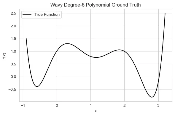
To evaluate the computational efficiency and sample effectiveness of each regression method, I designed a synthetic experiment involving a moderately complex nonlinear function.

This was done using a highly technical technique: button-mashing the Desmos online graphic calculator until it looked nice.

This function serves as a benchmark to test each model’s ability to learn expressive patterns under limited data settings:

$f(x) = 0.3x^6 - 2x^5 + 4x^4 - 1.3x^3 - 3.2x^2 + 2x + 1.$

Don’t worry, this is just a fancy way to describe a wiggly line that easily fits on a plot :)

import numpy as np

def true_function(x):
    return 0.3 * x**6 - 2 * x**5 + 4 * x**4 - 1.3 * x**3 - 3.2 * x**2 + 2 * x + 1

def noisy_function(x, noise_std=0.1):
    return true_function(x) + np.random.normal(0, noise_std, size=x.shape)

Success Criteria

We compare two regimes:

• Passive sampling: train on progressively larger random subsets of noisy samples
• Active sampling: let a GP choose the next samples using an acquisition policy (exploration/exploitation)

For each sample size we track:

• RMSE on a fixed test set
• Fit time per model

---

Models Definitions

Ridge as a strong baseline

In a traditional setting, linear models are optimized to reduce the residual sum of squares (RSS) across the dataset.

In theory, one could fit any nonlinear function using a flexible polynomial regressor.

This can negatively affect the model’s ability to generalize to unseen data by overfitting to the training set.

To reduce model complexity, regularization methods, such as Lasso (L1) and Ridge (L2) regression, are used.

In this case, we will focus on Ridge regression.

Ridge is fast and stable, especially with polynomial features.

It’s a great “first model” when you want a cheap baseline before reaching for heavier machinery.

from sklearn.pipeline import make_pipeline
from sklearn.preprocessing import PolynomialFeatures
from sklearn.linear_model import Ridge

ridge_model = make_pipeline(
    PolynomialFeatures(degree=6),
    Ridge(alpha=0.01),
)

SVR as the kernel middle-ground

Support vector machines (SVMs) are supervised learning models used in regression and classification tasks.

The attractiveness of SVMs comes from the fact that they are a sparse technique.

They rely solely on support vectors to make predictions rather than the entirety of the training set.

SVMs create convex optimization problems, even on nonlinear data, by using what is commonly known as the “kernel trick”.

Common kernels include linear, polynomial, sigmoid, and Gaussian radial basis functions (RBF).

In this paper, any reference to kernels will specifically pertain to the Radial Basis Function (RBF) kernel.

The choice is based on the RBF kernel being infinitely smooth, making it ideal for approximating complex unknown target functions.

The SVM projects the input space into a higher-dimensional feature space, which enables them to separate datasets that may initially appear to be linearly inseparable.

from sklearn.svm import SVR

svr_model = SVR(kernel="rbf", C=20, epsilon=0.005, gamma=1.0)

GPs: uncertainty + active sampling

Bayesian optimization techniques are often extremely sample-efficient due to their incorporation of prior beliefs, about the problem that directs sampling in an active setting rather than randomly or sequentially.

Bayesian linear regression is grounded in the theoretical concepts of Bayes’ rule.

It relies on the posterior distribution, $p(w \mid y,X)$, which is the product of the prior beliefs. $p(w)$, and likelihood, $p(y \mid X,w)$.

The two main components of a Bayesian optimization (BO) algorithm are the surrogate model and acquisition function.

The surrogate model is the model’s current “best guess” at estimating the objective function, and the acquisition function is the method by which we choose new locations to sample.

The most common surrogate model for continuous feature spaces is the Gaussian process (GP).

Similar to how a Gaussian distribution is a distribution over a random variable, the GP is a distribution over a function.

Instead of returning a scalar at some point $x$, the GP returns the mean and variance of a normal distribution over all possible values of $f(x)$ at $x$.

from sklearn.gaussian_process import GaussianProcessRegressor
from sklearn.gaussian_process.kernels import RBF, WhiteKernel

kernel = RBF(
  length_scale=1.5, length_scale_bounds=(0.3, 10.0)) + \
  WhiteKernel(noise_level=0.1, noise_level_bounds=(1e-4, 1.0)
)

gp_model = GaussianProcessRegressor(
  kernel=kernel,
  normalize_y=True,
  alpha=0.0,
  n_restarts_optimizer=10,
)

---

Results

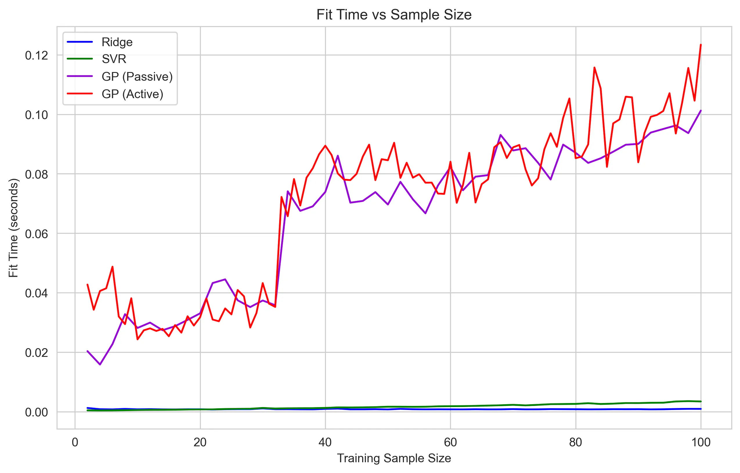
Computational Efficiency

The compute times seem to follow theoretical and practical expectations, in that:

Ridge and SVR remain extremely fast, while GP fit time grows dramatically as the kernel matrix scales.

Sample Efficiency

The sampling story is (unsurprisingly) the opposite:

The GP reaches strong performance with far fewer samples, especially with active sampling.

Although the Ridge regression is able to ultimately outperform both the SVR and GP, it takes far more samples to stabilize.

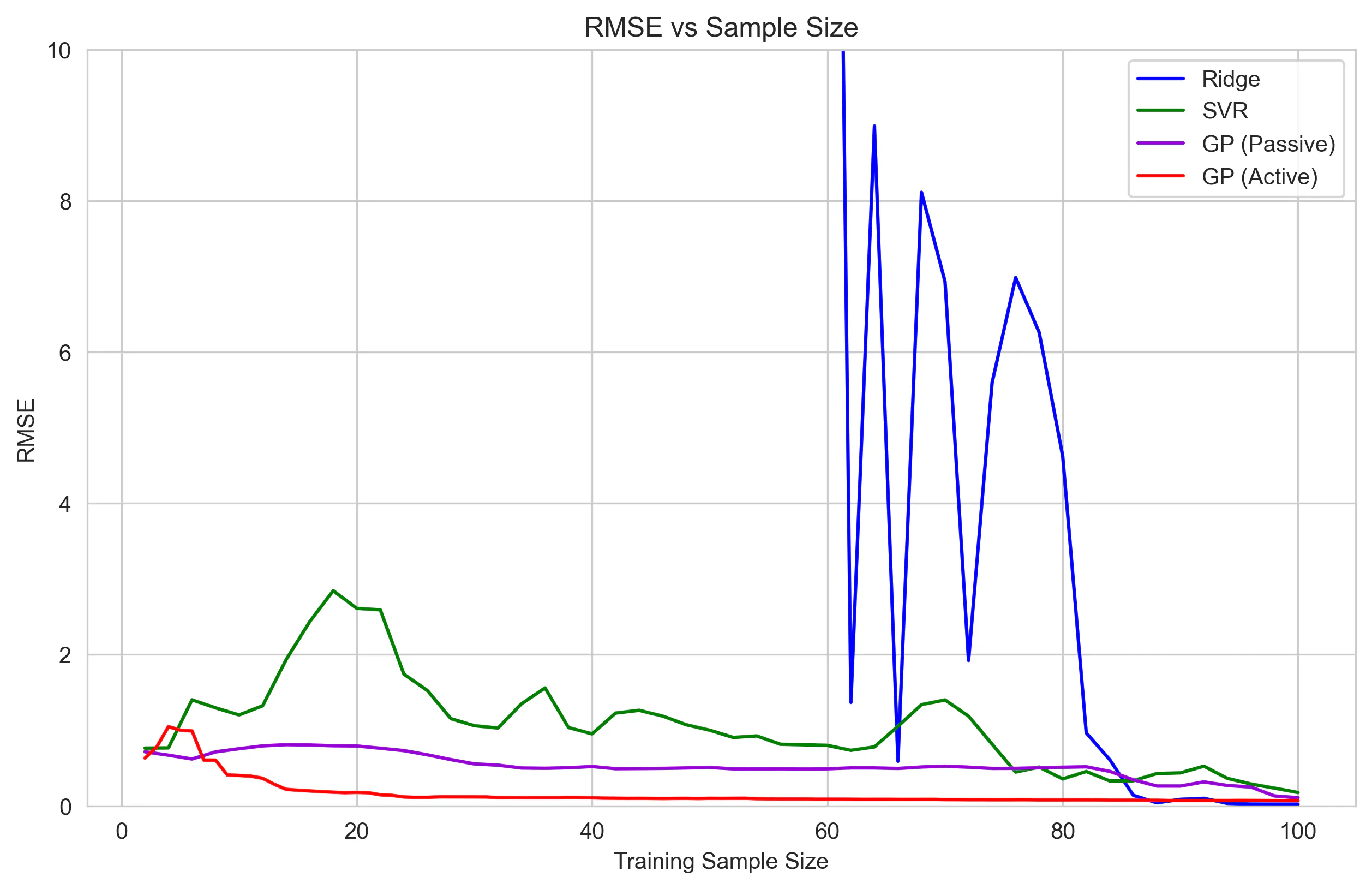
To make full use of the GP’s efficiency, we need to ask the question: how many samples is good enough?

The final figure aims to show how the acquisition-based sampling of the GP can reach high levels of performance with significantly fewer samples.

The red points on the scatter plot show the points that were sampled until the GP reached within 5% of the lowest RMSE of the SVM model after 100 samples.

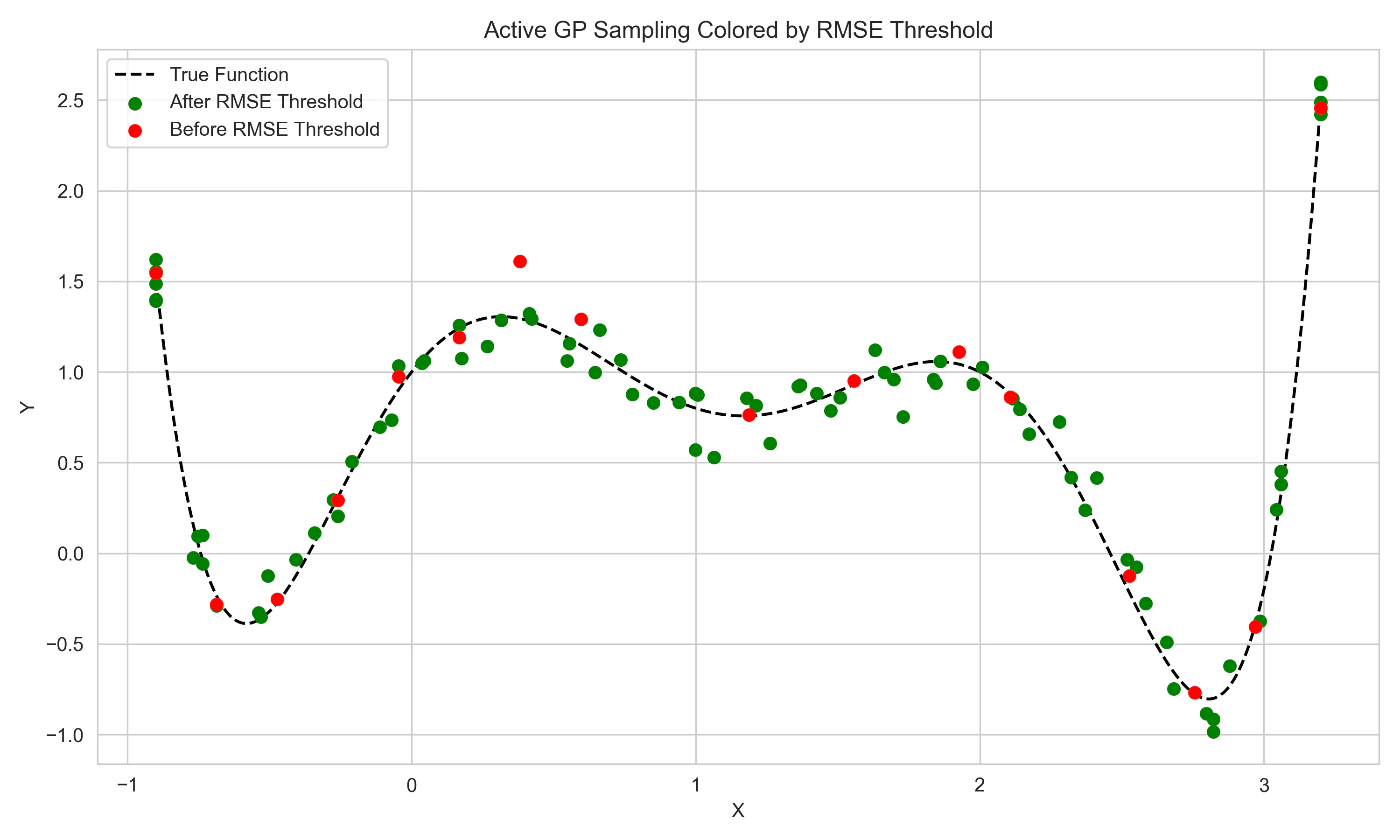
This threshold was hit after just 16 samples, 84% higher sample efficiency, emphasizing the powerful aspects of GPs in “expensive-to-evaluate” settings.

What this means in practice

• If your data is expensive, the GP can be worth it even if training is slower.
• If your data is cheap (or you already have a lot), Ridge/SVR often win on total cost.
• Active sampling is where the GP becomes a different kind of tool: not just a regressor, but a data-collection strategy.